The Independent Chip Model (ICM): Foundations, Calculation, Applications, and Limitations

The Independent Chip Model (ICM) is the most widely adopted framework for valuing tournament chips in poker. Unlike cash games, where chips have linear monetary value, tournament chips represent probabilistic equity in a non-linear prize distribution. This article presents a comprehensive overview of ICM: its historical origins, mathematical foundations, calculation procedures, strategic applications, and limitations. We further discuss extensions such as the Malmuth-Harville model, Future Game Simulation (FGS), and Nash ICM. By situating ICM within both mathematical probability theory and human decision-making biases, we provide an integrative account of why ICM is both indispensable and flawed in practice.

1. Introduction

Tournament poker introduces a fundamental problem of valuation: what is a chip worth? In a cash game, the answer is trivial—chips are fungible with money at a one-to-one ratio. In tournaments, however, chips serve only as a representation of survival and relative standing in pursuit of non-linear payout structures.

For example, consider a tournament with 100 entrants, each paying $100, generating a $10,000 prize pool. The typical payout structure may award $3,000 to the winner, $2,000 to the runner-up, $1,500 to third, and so on. In this context, doubling one’s stack does not double expected prize equity, because chip utility depends on tournament stage and payout curve.

The Independent Chip Model (ICM) emerged in the early 2000s as the dominant approach to solve this problem. Originally proposed in poker forums and refined by theorists such as Mason Malmuth, ICM remains the gold standard for calculating tournament equity.

2. Conceptual Foundations

The Independent Chip Model is built upon two conceptual assumptions:

Chips determine probability of finishing positions.
Each player’s probability of winning first place is proportional to their share of total chips.
Recursive calculation of subsequent positions.
After assigning first place, probabilities for remaining positions are calculated by removing the winning stack and renormalizing the remaining chips (Malmuth & Harville, 2001).

This recursive framework produces, for every player, a probability distribution over finishing positions. Multiplying these probabilities by the prize structure yields expected monetary equity.

ICM assumes all players are of equal skill and that chips are played independently of future position or blind pressure—assumptions that simplify reality but enable tractable calculations.

3. Mathematical Formulation

Let:

$N$ = number of players remaining,
$C_i$ = chip count of player $i$,
$T = \sum_{i=1}^N C_i$ = total chips in play,
$P_j$ = prize for finishing in position $j$.

Step 1: Probability of winning first place $$\Pr(\text{Player } i \text{ finishes 1st}) = \frac{C_i}{T}$$

Step 2: Probability of finishing in later positions

For second place, conditional probabilities are calculated by removing the first-place player and normalizing remaining stacks:

$$\Pr(\text{Player } i \text{ finishes 2nd}) = \sum_{k \neq i} \Pr(k \text{ finishes 1st}) \cdot \frac{C_i}{T – C_k}$$

This process continues recursively until all finishing positions are assigned probabilities.

Step 3: Recursive continuation
This process continues recursively until all positions are exhausted.

Step 3: Equity calculation

Expected monetary equity for player $i$ is:

$$E_i = \sum_{j=1}^N \Pr(\text{Player } i \text{ finishes in position } j) \cdot P_j$$

4. Worked Example (3 Players)

Consider three players with chip counts:

A = 5000, B = 3000, C = 2000. Total = 10,000.
Payouts: 1st = $50, 2nd = $30, 3rd = $20.

Step 1: First-place

A: 0.50, B: 0.30, C: 0.20.

Step 2: Second-place

If A wins: B = 0.60, C = 0.40.
If B wins: A ≈ 0.714, C ≈ 0.286.
If C wins: A = 0.625, B = 0.375.

Weighted averages yield:

A second ≈ 0.325, B second ≈ 0.362, C second ≈ 0.313.

Step 3: Final equities

A ≈ $42.5, B ≈ $32.1, C ≈ $25.4.

Player	Chip Count	Chip %	ICM Equity ($)
A	5000	50,0%	42,5
B	3000	30,0%	32,1
C	2000	20,0%	25,4

Table 1: ICM Example: Chip Counts vs. Equity

Despite holding 50% of chips, A’s equity is less than 50% of the prize pool—a hallmark of ICM’s non-linear valuation.

5. Applications in Tournament Poker

5.1 Bubble Play

Near the payout threshold (“the bubble”), chip preservation outweighs chip accumulation. ICM predicts that medium stacks should play conservatively, while large stacks exploit by applying pressure.

5.2 Final Table Strategy

ICM equity often dictates folds of hands that would be calls in cash games. The so-called “ICM tax” reflects the asymmetric risk of elimination (Sklansky, 1999).

5.3 Deal-Making

ICM is the industry standard for final table deals. Tournament directors often use ICM-based calculations to divide prize pools equitably (Harrington & Robertie, 2005).

Figure 2
Chip Share vs. ICM Equity Share
Comparison of chip percentages versus ICM equity percentages for three players. The figure illustrates how Player A’s equity falls below chip share, while Players B and C gain relative equity.

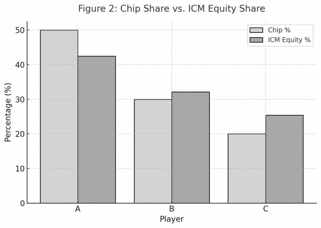
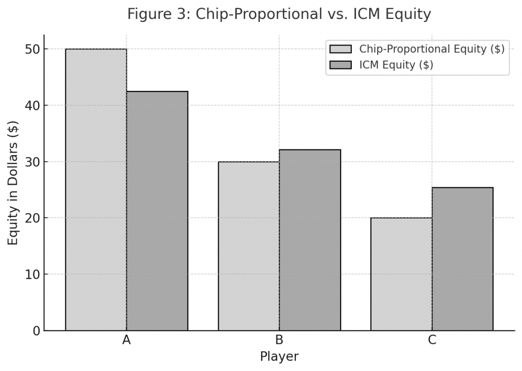
Figure 3
Chip-Proportional vs. ICM Equity in Dollars
A bar chart contrasting hypothetical chip-based payouts with ICM-calculated equities. Demonstrates the non-linear valuation of tournament chips.

6. Limitations of ICM

Equal-skill assumption: ICM ignores differences in ability. A world-class player and a novice with equal stacks are assigned identical equities.
No future game modeling: Blind levels, positional effects, and future shove/fold dynamics are excluded.
Over-simplification in multiway pots: ICM assumes independence, yet real play involves complex interactions.
Non-robustness at extreme stacks: Very short or very large stacks may behave differently than ICM predicts (Miller, 2007).

7. Extensions Beyond ICM

Malmuth-Harville Model (MHM): A refinement incorporating finish-order probability modeling from horse racing statistics.
Future Game Simulation (FGS): Extends ICM by simulating future hands, blind increases, and stack dynamics (Larkey et al., 1997).
Nash ICM: Combines ICM with Nash equilibrium shove/fold strategies to model equilibrium play at short stacks (Chen & Ankenman, 2006).

These models attempt to bridge the gap between theoretical elegance and real-world dynamics.

8. Psychological and Behavioral Perspectives

From a cognitive science perspective, ICM illustrates how human intuition about probabilities often deviates from mathematical models. Players tend to overvalue chip accumulation and undervalue survival, consistent with prospect theory and risk asymmetry. Understanding ICM not only sharpens poker strategy but also highlights broader limitations in human probabilistic reasoning.
Cognitive biases such as the gambler’s fallacy and overconfidence further distort tournament decisions (Barberis, 2013).

9. Conclusion

The Independent Chip Model remains a cornerstone of tournament poker analysis. Its recursive probability framework captures the nonlinear relationship between chips and prize money, influencing strategy, bubble play, and deal-making. Despite limitations, ICM provides a practical and widely accepted tool for decision-making under uncertainty. Extensions such as FGS and Nash ICM continue to evolve the model, bringing it closer to real tournament conditions.

Understanding ICM is not only essential for competitive poker players but also offers insights into applied probability, risk management, and human decision-making under uncertainty.

References

Barberis, N. (2013). Thirty years of prospect theory in economics: A review and assessment. Journal of Economic Perspectives, 27(1), 173–196.
Chen, B., & Ankenman, J. (2006). The Mathematics of Poker. ConJelCo.
Harrington, D., & Robertie, B. (2005). Harrington on Hold’em: Volume II. Two Plus Two Publishing.
Kahneman, D., & Tversky, A. (1979). Prospect theory: An analysis of decision under risk. Econometrica, 47(2), 263–291.
Larkey, P. D., Kadane, J. B., Austin, R. H., & Zamir, S. (1997). Skill in games. Management Science, 43(5), 596–609.
Malmuth, M., & Harville, D. A. (2001). Probability models and poker tournament equity. Two Plus Two Publishing.
Miller, E. (2007). Tournament Poker for Advanced Players. Two Plus Two Publishing.
Sklansky, D. (1999). The Theory of Poker. Two Plus Two Publishing.